Finding Donors For CharityML
· 15 min read
· 15 min read

This project employs several supervised algorithms to accurately model individuals’ income using data collected from the 1994 U.S. Census. The best candidate algorithm is chosen from preliminary results and further optimized to best model the data. The goal of this implementation is to construct a model that accurately predicts whether an individual makes more than $50,000. This sort of task can arise in a non-profit setting, where organizations survive on donations. Understanding an individual’s income can help a non-profit better understand how large of a donation to request, or whether or not they should reach out to begin with. While it can be difficult to determine an individual’s general income bracket directly from public sources, this value can be inferred from other publically available features.
The dataset for this project originates from the UCI Machine Learning Repository. The datset was donated by Ron Kohavi and Barry Becker, after being published in the article “Scaling Up the Accuracy of Naive-Bayes Classifiers: A Decision-Tree Hybrid”. The article by Ron Kohavi can be found online. The data investigated here consists of small changes to the original dataset, such as removing the 'fnlwgt' feature and records with missing or ill-formatted entries.
A cursory investigation of the dataset determined how many individuals fit into either group, and revealed the percentage of individuals that makes more than $50,000. Of the 45,222 individuals which make up the dataset, 11,208 (24.78%) of the individuals makes more than $50,000, while 34014 individuals makes at most $50,000.
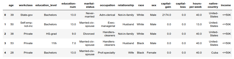
The following features are available in the dataset:
Before data can be used as input for machine learning algorithms, it often must be cleaned, formatted, and restructured — this is typically known as preprocessing. Fortunately, for this dataset, there are no invalid or missing entries. However, there are some qualities about certain features that need to be adjusted. Preprocessing can help tremendously with the outcome and predictive power of nearly all learning algorithms.
A dataset may sometimes contain at least one feature whose values tend to lie near a single number, but will also have a non-trivial number of vastly larger or smaller values than that single number. Algorithms can be sensitive to such distributions of values and can underperform if the range is not properly normalized. With the census dataset two features fit this description: 'capital-gain' and 'capital-loss'.
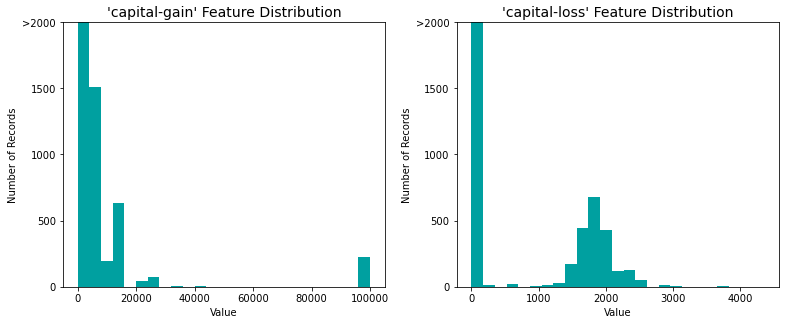
For highly-skewed feature distributions such as 'capital-gain' and 'capital-loss', it is common practice to apply a logarithmic transformation on the data so that the very large and very small values do not negatively affect the performance of a learning algorithm. Using a logarithmic transformation significantly reduces the range of values caused by outliers. Care is taken when applying this transformation however: The logarithm of 0 is undefined, so the values are translated by a small amount above 0 to apply the logarithm successfully.
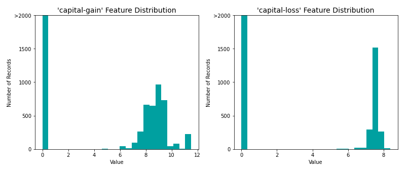
In addition to performing transformations on features that are highly skewed, numerical features are normalized as it is often good practice to perform some type of scaling on numerical features. Applying a scaling to the data does not change the shape of each feature’s distribution (such as 'capital-gain' or 'capital-loss' above); however, normalization ensures that each feature is treated equally when applying supervised learners.
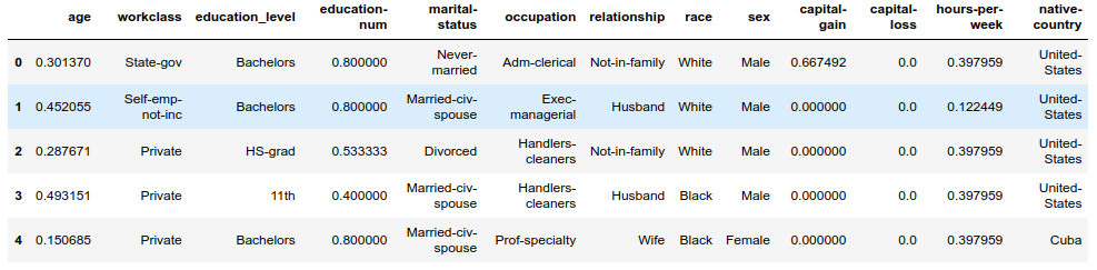
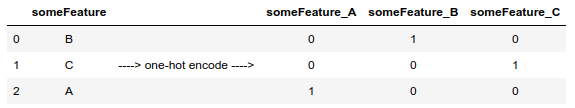
There are several features for each record that are non-numeric, as pointed out in Data Exploration above. Typically, learning algorithms expect input to be numeric, which requires that non-numeric features (called categorical variables) be converted. One popular way to convert categorical variables is by using the one-hot encoding scheme.
One-hot encoding creates a “dummy” variable for each possible category of each non-numeric feature. For example, assume someFeature has three possible entries: A, B, or C. This can be encoded into someFeature_A, someFeature_B and someFeature_C.
Additionally, as with the non-numeric features, the non-numeric target label, 'income' is converted to numerical values for the learning algorithm to work. Since there are only two possible categories for this label (“<=50K” and “>50K”), it is simply encoded as 0 and 1, respectively.
After all categorical variables are converted into numerical features, and all numerical features normalized, the data - both features and their labels - are split into training and test sets. The splits are 80% of the data for training and 20% for testing.
Four different algorithms are investigated to determine the best at modeling the data. Three of these are supervised learners, and the fourth algorithm is a carefully selected naive predictor.
CharityML, equipped with their research, knows individuals that make more than $50,000 are most likely to donate to their charity. Because of this, CharityML is particularly interested in predicting who makes more than $50,000 accurately. It would seem that using accuracy as a metric for evaluating a particular model’s performace would be appropriate. Additionally, identifying someone that does not make more than $50,000 as someone who does would be detrimental to CharityML, since they are looking to find individuals who are willing to donate.
Accuracy measures how often the classifier makes the correct prediction. Precision measures what proportion of individuals classified as making more than $50,000, actually makes more than $50,000. While Recall measures what proportion of individuals that actually makes more than $50,000 is classified as making more than $50,000. Therefore, a model’s ability to precisely predict those that make more than $50,000 is more important than the model’s ability to recall those individuals.
F-beta score is a metric that considers both precision and recall:
\[F\_{\beta} = (1 + \beta^2) \cdot \frac{precision \cdot recall}{\left( \beta^2 \cdot precision \right) + recall}\]In particular, when $\beta = 0.5$, more emphasis is placed on precision. This is called the F$_{0.5}$ score (or F-score for simplicity). This score can range from 0 to 1, with 1 being the best possible score.
Looking at the distribution of classes (those who make at most \$50,000, and those who make more), it is clear that most individuals do not make more than $50,000. This can greatly affect accuracy, since it could simply be said that “this person does not make more than $50,000” and generally be right, without ever looking at the data! Making such a statement would be called naive, since no information was considered to substantiate the claim. It is always important to consider the naive prediction for data, to help establish a benchmark for whether a model is performing well. That been said, using that prediction would be pointless: If the algorithm predicted all people makes less than $50,000, CharityML would identify no one as donors.
The the purpose of generating a naive predictor is simply to show what a base model without any intelligence would look like. In the real world, ideally the base model would be either the result of a previous model or could be based on a research paper with room for improvement. Since there is no benchmark model set, getting a result better than random choice is a good start.
If a model that always predicts an individual makes more than $50,000 is chosen, what would that model’s accuracy and F-score be on this dataset?
It can simply be deduced that the naive predictor accuracy equals it’s precision. A model that always predicts ‘1’ - positive - (i.e. the individual makes more than 50k) will have no True Negatives (individuals that makes at most 50k classified as making at most 50k) or False Negatives (individuals that makes at most 50k classified as making more than 50k) as it is not making any ‘0’ - negative - predictions. Therefore its’ Accuracy in this case becomes the same as its’ Precision as every true prediction that should be false becomes a False Positive.
The Naive Predictor applied on the census data has an Accuracy score of 0.2478, and a F-score of 0.2917.
The following models are considered for this analysis: Logistic Regression, Support Vector Machines, and Ensemble Methods.
The Logistic Regression model is a linear classifier that estimates the probability of an event (such as testing positive or negative) based on a linear combination of one or more independent variables. It is easy to set up, train, and interpret, and performs well when the classes are linearly separable. One limitation however, is that it is not flexible enough to capture complex relationships and performs poorly when there are multiple or non-linear decision boundaries. But because of its simplicity and interpretability, it is a good starting point for binary classification problems.
Support Vector Machines are a group of supervised learning models that can be used for both classification and regression problems. They perform well in high-dimensional spaces and can scale to large number of samples. The workings of SVMs are not easily interpretable because of their algorithmic complexities, but their inherent two-class nature makes them suitable for problems involving binary classification.
Ensemble methods such as Gradient Boost and Random Forests combine simple learners — i.e., decision trees — to create a more robust learner. They perform very well as decision trees can learn non-linear relationships but they take longer to train. They can also handle imbalances in datasets and the hierarchical structure of their trees makes them perform well in binary classification problems.
The three models - with their default parameters - are trained on 1%, 10%, and 100% of the training data.
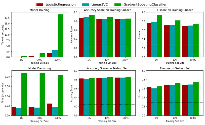
Figure 3 visualizes the performance of the three supervised learning models. Because the goal is to precisely identify the category with income greater than $50,000 and to recall a significant number of individuals in that category, the F score evaluation is given more attention since it best captures this situation. It is tuned to favor precision.
From the figure, GradientBoostingClassifier outperforms the other models when all of the data is used for training. Although the model takes much longer to train, the prediction time is relatively short. The longer training time is due to the model’s individual decision trees being built sequentially. This sequential addition produces a robust predictor even when there is an imbalance of classes in the data. It performs well in this situation given that the number of features are relatively low.
It is possible and recommended to search a models’ hyper-parameter space for optimal values in order to improve its predictive performance — this is typically known as model tuning. One popular way to tune a Gradient Boosting Classifier is by using GridSearch. GridSearch exhaustively generates candidates from a grid of hyper-parameter values, evaluates all possible combinations and retains the best one. It is performed on the untuned model over the entire training set in order to improve its F-score.
Additionaly, Early Stopping support in Gradient Boosting enables building a model that generalizes well to unseen data using the least number of iterations. Using fewer iterations can siginificantly reduce a models training time. Combination of gridsearch and early stopping produces an optimized model to be used on the Census Data.
Table 4 presents a side by side comparison of the performance metrics of the unoptimized and optimized model. The optimized GradientBoostingClassifier achieves an accuracy of 86.77% and an F-score of 74.57%, both of which are slightly higher than the scores of the unoptimized model. Applying early stopping reduced the overall training time from 21.27 seconds to 12.08 seconds. Considering this, the scores of the optimized model are better than the unoptimized model.
| Metric | Unoptimized Model | Optimized Model |
|---|---|---|
| Accuracy Score | 0.8630 | 0.8677 |
| F-score | 0.7395 | 0.7457 |
| Train Time | 21.27 | 12.08 |
Furthermore, comparing with the Naive Predictor, it outperforms the naive predictor benchmarks by a wide margin. The accuracy increased by about 72%, with a 61% increase in F-score.
An important task when performing supervised learning on a dataset like the census data is determining which features provide the most predictive power. By focusing on the relationship between only a few crucial features and the target label, understanding of the phenomenon can be simplified, which is almost always a useful thing to do. In the case of this project, that means to identify a small number of features that most strongly predicts whether an individual makes at most or more than $50,000.
Knowing the importance of features as indicated by machine learning models can be beneficial. By gaining a better understanding of the models’ logic, the correctness of its results can be verified . The key features can also be used in variable selection and the model can be improved by focusing only on the key variables. As a result, the interpretability of the model’s decision becomes easier.
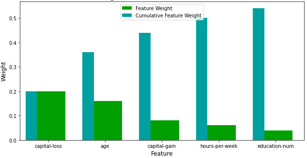
In Exploring the Data, it was shown there were thirteen available features for each individual on record in the census data. Of these thirteen records, the following five features are considered - by observation - to be most important for prediction, and are ranked in the order listed with reasons discussed.
Capital-loss: This is likely the most important factor in predicting if an individual makes at most or above $50,000 considering that net income is greatly affected by losses. Whether an individual has a fixed salary or earns commissions on product sales, their overall income is determined by how much money they lose.
Captal-gain: For similar reasons as above, capital gain is ranked second.
Occupation: Because a person’s income is based on the skills required for a particular profession, I believe occupation is the third most essential feature in determining a person’s income. Positions requiring more technical and organizational skills typically pay more than jobs requiring less.
Education: Education is placed fourth because, while school broadens one’s knowledge base, most occupations require skills that can be acquired through skill acquisition programs or trainings that are not part of a traditional education.
Hours-per-week: Lastly, while hours are a significant aspect, it is not the most deciding criterion among the five outlined, because working longer hours does not always imply making more money.
Looking at figure 4, capital-loss is the most important factor in predicting whether an individual makes at most or above \$50,000, as presumed, and hours-per-week is also ranked low, as expected. However, age, appears to play a substantial role in the prediction, which was not previously considered as a factor in predicting an individual’s income. In terms of education-num as a factor, it was assumed that education would be more appropriate in this situation. Excluding these differences, the features chosen by the machine learning model are relatively similar to what was considered to be the most important in determining whether an individual makes at most or above $50,000.
How does a model perform if we only use a subset of all the available features in the data?
With less features required to train, the expectation is that training and prediction time will be much lower — at the cost of the performance metrics. From the visualization above, the top five most important features contribute more than half of the importance of all features present in the data. This hints that an attempt can be made to reduce the feature space and simplify the information required for the model to learn.
Table 5 presents the results of training the optimized model on the same training set with only the top five important features.
| Metric | All Features | Top 5 Features Only |
|---|---|---|
| Accuracy Score | 0.8677 | 0.8409 |
| F-score | 0.7457 | 0.6937 |
Training on the reduced data yields lower scores than training on the full data. There is a 2.68% difference in accuracy but this is less significant compared to the 5.2% difference in F-score. Because F-score is biased towards the model’s precision, the model trained on the reduced data would misidentify more people as belonging to the group making more than $50,000. But, however, considering only a subset of the features were used in training, it performs remarkably. This illustrates the importance of feature selection as well as its contribution to the model’s overall predicting performance. If training time was a consideration, It would be beneficial to use the reduced data as the training set since the model’s performance on training with the reduced data is significantly better than naive prediction, and nearly as good as the optimized model.