The Oxford 102 Flowers
· 3 min read
· 3 min read

Going forward, AI algorithms will be incorporated into more and more everyday applications. A large part of software development in the future will use deep learning models trained on hundreds of thousands of images as part of their overall application architecture. This project trains an image classifier to recognize different species of flowers. An example application might be a phone app that tells the name of the flower a camera is looking at.
This project has two parts:
The dataset for this project is the Oxford 102 Category Flower Dataset compiled by Maria-Elena Nilsback and Andrew Zisserman, and published in their article “Automated Flower Classification Over a Large Number of Classes”. The article can be found here.
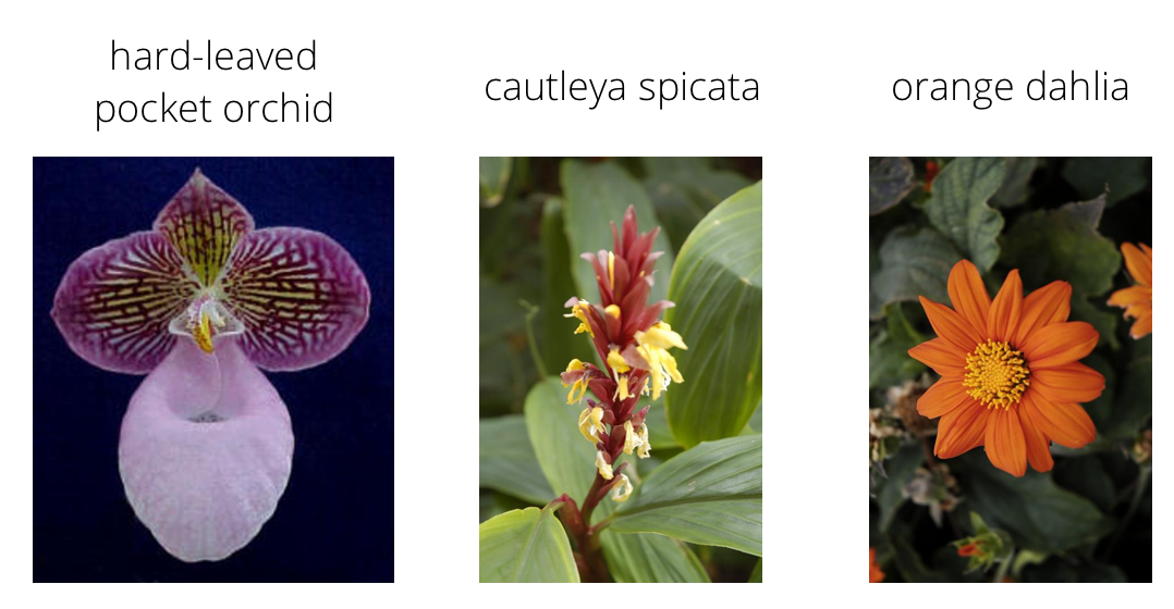
The Dataset comprises of 102 flower categories commonly occurring in the United Kingdom. Each category contains between 40 and 258 images with different variations - large scale, pose and light. A few of the images with thier labels are shown below.
The dataset has 3 splits: 'train', 'test', and 'validation'. The train set is used to train the model while the validation and test sets are used to measure the model’s performance on data it hasn’t seen yet.
The train and validation sets each contain 1020 images each (10 images per class), and the test set contains 6149 images (minimum 20 per class), making a total of 8189 images in the dataset.
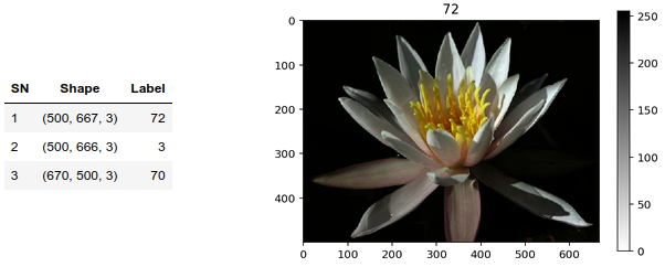
The figure below shows the shape of 3 images in the dataset with one of the images displayed. As can be seen, the raw images have a variety of sizes with three color channels each. Each pixel value in the images are in the range [0, 255].
Deep neural networks process data in batches. The batch size is the number of images that the neural network receives in one iteration. This neural network expects the images in the batch to be consistent in their shapes and sizes. It was shown previously that the images in the dataset are of different shapes. These images need to be standardized to a fixed size. In addition, the network expects the pixel values of the images to be in the range [-1, 1], but the images in the dataset are in the range [0, 255]. These will have to be normalized.
A pipeline is a set of transformations that is applied to the data so that it can be fed efficiently to the network. Achieving peak performance requires an input pipeline that delivers the batch for the next iteration before current iteration completes.
A pipeline is created to cache and prefetch the batches, optimizing their loading speeds. It loads the images in batch sizes of 32, standardizes the images to the shape (224x224), and normalizes the pixel values in the range [-1, 1].
Convolutional Neural Networks are best for image classification. However, Modern CNNs have millions of parameters. Training them from scratch will require a ton of computing power (hundreds of gpu hours or more). Because such resources are unavailable and the goal is to spend less time building the classifier, a pre-trained neural network is leveraged and adapted to the new dataset - this is known as transfer learning. Transfer learning often includes additional training and or fine tuning depending on both the size of the new dataset, and, the similarity of the new dataset to the original dataset.
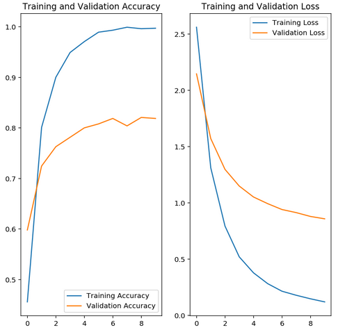
MobileNet pre-trained network is used for extracting the features from the images. A new untrained feed-forward classifier is added to the MobileNet pre-trained network and the classifier is trained for 10 epochs using ‘Adam’ optimization. The plot below shows the loss and accuracy values achieved during training for the train and validation set.
It is good practice to test the trained network on test data, images the network has never seen either in training or validation. This will provide a good estimate for the model’s performance on completely new images. If the model has been trained well, it should be able to reach around 70% accuracy on the test set. The trained model achieved a 77.38% accuracy on the test set with a loss of 0.98.
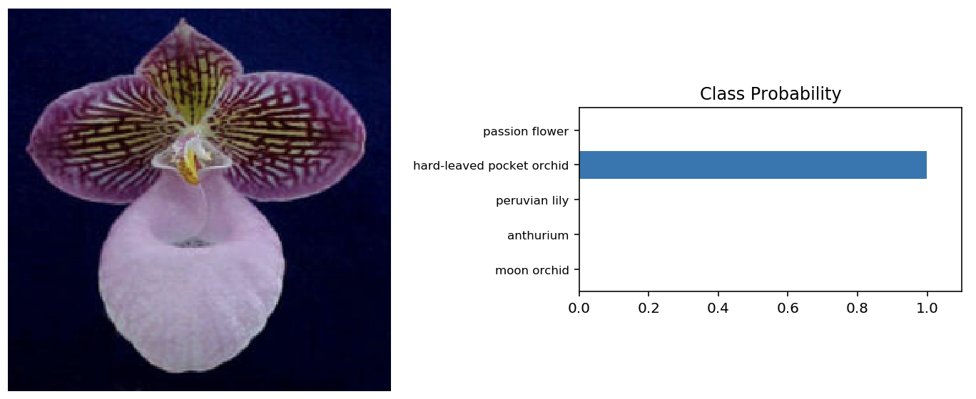
It’s always good to check the predictions made by the model to make sure they are correct. To check the predictions, the model is tested with 4 random images. The plot shows one input image alongside the probabilities for the top 5 classes predicted by the model as a bar graph.
This fufilled the requirement.Thus, the model is saved for use in the command-line application.